8.2 - Optimization and discounting

Change the model to take into account the growing future demand and therefore a higher future price for the resource. Introduce another parameter which will describe the growing demand for the resource. Make the price a function of both demand and supply. How does this change the results of optimization? Does the discounting still play an important role?

I assumed demand growth independent of supply or price according to the equation

demand = .5*exp(0.15*TIME)

I incorporated demand into price by changing the price function to

price = a*demand/(1 + mining) + b

The major effect on optimization was to increase the value of d from 2.36 to 3.01, which represents more rapid changes in rate of mining.

Discounting plays a more important role than without the growth in demand. The following table summarizes the effects of demand growth and discounting.

Total profits

Discount rate:	0%	5%
No demand function	$105k	$66k
Growing demand	$699k	$68k

Exhaustion of resource. Time to exhaustion or, if no exhaustion, resource remaining after 50 years

Discount rate:	0%	5%
No demand function	after 50y, 2.7 remain	20.7y
Growing demand	after 50y, 80 remain	20.2y

Discounting clearly drives much faster extraction of the resource, and, at least as I formulated the demand function, growing demand has little consequence in a 5% discount rate world -- the urgency of getting the resource to market to be able to take advantage of the discount rate seems to dominate the system.

8.1 - Optimization, abstractly

1. Imagine that your system is an airplane and you need to land it. Formulate and optimization task that will allow you to safely touch the ground at the airport nearby. What is the objective function? What are the control parameters, and the restrictions?

The optimization task is to bring the plane to height = 0 at the location of the runway, with the plane's vector parallel with the runway and the change in altitude of the plane as close to zero as possible.

The objective function is the change in altitude of the plane at the time of contact. The control parameters are the speed and course of the plane leading up to landing. The constraints are the location and direction of travel of the plane at the time of landing.

2. Think of an optimization of your own. Define the system, the objective function, the controls and restrictions.

Let's say we want to optimize the hydrology below a surface mine. The system includes precipitation, upland runoff, the topography, geology, and vegetation of the mine, and the topography, geology, and ecology--including, potentially, humans--below the mine.

Let's make the objective function the difference between post-mining flow and pre-mining flow. The controls include placement of overburden, compaction of replaced topsoil, vegetation planted, and potential settling ponds and/or dykes downstream of the mine. The constraints include the surrounding topography, precipitation and other climatic variables, and upstream hydrology.

7.4 - Supply & Demand Equilibrium via Price

If we assume that the growth in Supply and Demand is defined by Price, whereas the decline of Supply is determined by Demand and the decline in Demand is determined by Supply directly, we come up with a model that produces some strange dynamics. Try to figure out what causes this strange dynamics. What are the other possible trajectories that may be generated? Is there an equilibrium? 

It seems that delays cause the wonky behavior. Notice that as demand rises, price rises but lag behind. And as price starts to rise, supply is still falling. It looks like the slope of supply is driven by the inflection of price. That is, when the second derivative of the price function is negative, supply falls, whether price is increasing or decreasing. But I think that in the market, as price falls, regardless of its second derivative, supply would also fall.

By removing the direct informational link between supply and demand; that is, with price as their only intermediary, the behavior generated is similar to that of the predator-prey system from the chapter before last. There's no equilibrium here, because there's no mechanism for supply or demand to fall we just get continuous growth.

7.3 - Price/quantity model

Put together the Price - Goods model in Stella or download it from here. Try to find another function or set of parameters that would make it converge faster.

I tweaked the parameters and production/consumption functions and to get faster convergence. I ended up with the following parameters and functions:

C_g1 = 0.02
C_g2 = 0.03
C_p1 = 0.0055
C_p2 = .06
Production = C_g1*Price^1.55
Consumption = 1/C_g2/Price^0.25

Old

New

7.2 - Human population model with economic data

I built a new model for this exercise but kept the immigration and emigration graphical functions from the last exercise because they don't relate in any obvious way to time or prosperity. I modeled per capita GDP as a function of time: GDP = 1.826*e ^ (.02*t) where t = year with 1851 = 0. I developed that equation from a quick web search for historical economic data. I then modeled natality and mortality as functions of per capita income: natality = 0.0507*GDP^-0.34 and mortality = 0.0268*GDP^-0.377. Here is the result:

7.1 - Human Population Model

Try to improve the calibration of the population model by further modifying the parameters a₁ and a₂. You can either continue the trial and error exercises or upload the model into Madonna and try the curve-fitting in there. Do not forget to add the Error function to the model since visual comparison becomes quite hard once we get really close to the optimal solution. Is there a better combination of parameters than a₁ = a₂ = 0.1? 

I  tried messing with the coefficients quite a bit, and I get the best performance with ain = 0.1 and aout = 0.11. The pink line is the error function, defined as 100*(Population-DATA)/Population.

Ex 6.6 - Global hydrological model

1. What modifications should be made to the conceptual model if a time scale of 1 year and a spatial scale of 1 km² are chosen for the model? What processes can be excluded? simplified? described in more detail? 

The elevation aspect of the model can be excluded; it is important when there is flow between adjacent cells, but if we're just modeling a single area, it is irrelevant. The climatic data, on the other hand, could be made more precise, both temporally and spatially.

2. Compare dry year (halved precipitation) and wet year (doubled precipitation) dynamics within the model. Does the model produce reasonable estimates for the state variables? Does it tend to an equilibrium if such conditions prevail, or it shows a trend over several years? 

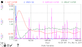
It does reach an equilibrium, and equilibrium levels of saturated water and unsaturated water are remarkably similar despite the four-fold difference in precipitation. What does change quite significantly is the amount of surface water (and snowpack):

Half precipitation

1x precipitation

Double precipitation

 The same patterns and equilibria hold when the simulation is run over three years.

3. Can you find a parameter in this model, modifying which you can produce a trend over several years that destabilizes the system?

First of all, I love these how-to-break-the-system questions.

Second, if we're given sufficient latitude with the parameters, the question becomes rather simple. Increasing transpiration potential by a factor of ten does little to the system; it remains stable at a very similar equilibrium; however, increasing the same parameter by a factor of 1000 sucks all the water right out of the system:

1000-fold increasing in transpiration potential