8.2 - Optimization and discounting

Change the model to take into account the growing future demand and therefore a higher future price for the resource. Introduce another parameter which will describe the growing demand for the resource. Make the price a function of both demand and supply. How does this change the results of optimization? Does the discounting still play an important role?

I assumed demand growth independent of supply or price according to the equation

demand = .5*exp(0.15*TIME)

I incorporated demand into price by changing the price function to

price = a*demand/(1 + mining) + b

The major effect on optimization was to increase the value of d from 2.36 to 3.01, which represents more rapid changes in rate of mining.

Discounting plays a more important role than without the growth in demand. The following table summarizes the effects of demand growth and discounting.

Total profits

Discount rate:	0%	5%
No demand function	$105k	$66k
Growing demand	$699k	$68k

Exhaustion of resource. Time to exhaustion or, if no exhaustion, resource remaining after 50 years

Discount rate:	0%	5%
No demand function	after 50y, 2.7 remain	20.7y
Growing demand	after 50y, 80 remain	20.2y

Discounting clearly drives much faster extraction of the resource, and, at least as I formulated the demand function, growing demand has little consequence in a 5% discount rate world -- the urgency of getting the resource to market to be able to take advantage of the discount rate seems to dominate the system.

8.1 - Optimization, abstractly

1. Imagine that your system is an airplane and you need to land it. Formulate and optimization task that will allow you to safely touch the ground at the airport nearby. What is the objective function? What are the control parameters, and the restrictions?

The optimization task is to bring the plane to height = 0 at the location of the runway, with the plane's vector parallel with the runway and the change in altitude of the plane as close to zero as possible.

The objective function is the change in altitude of the plane at the time of contact. The control parameters are the speed and course of the plane leading up to landing. The constraints are the location and direction of travel of the plane at the time of landing.

2. Think of an optimization of your own. Define the system, the objective function, the controls and restrictions.

Let's say we want to optimize the hydrology below a surface mine. The system includes precipitation, upland runoff, the topography, geology, and vegetation of the mine, and the topography, geology, and ecology--including, potentially, humans--below the mine.

Let's make the objective function the difference between post-mining flow and pre-mining flow. The controls include placement of overburden, compaction of replaced topsoil, vegetation planted, and potential settling ponds and/or dykes downstream of the mine. The constraints include the surrounding topography, precipitation and other climatic variables, and upstream hydrology.

7.4 - Supply & Demand Equilibrium via Price

If we assume that the growth in Supply and Demand is defined by Price, whereas the decline of Supply is determined by Demand and the decline in Demand is determined by Supply directly, we come up with a model that produces some strange dynamics. Try to figure out what causes this strange dynamics. What are the other possible trajectories that may be generated? Is there an equilibrium? 

It seems that delays cause the wonky behavior. Notice that as demand rises, price rises but lag behind. And as price starts to rise, supply is still falling. It looks like the slope of supply is driven by the inflection of price. That is, when the second derivative of the price function is negative, supply falls, whether price is increasing or decreasing. But I think that in the market, as price falls, regardless of its second derivative, supply would also fall.

By removing the direct informational link between supply and demand; that is, with price as their only intermediary, the behavior generated is similar to that of the predator-prey system from the chapter before last. There's no equilibrium here, because there's no mechanism for supply or demand to fall we just get continuous growth.

7.3 - Price/quantity model

Put together the Price - Goods model in Stella or download it from here. Try to find another function or set of parameters that would make it converge faster.

I tweaked the parameters and production/consumption functions and to get faster convergence. I ended up with the following parameters and functions:

C_g1 = 0.02
C_g2 = 0.03
C_p1 = 0.0055
C_p2 = .06
Production = C_g1*Price^1.55
Consumption = 1/C_g2/Price^0.25

Old

New

7.2 - Human population model with economic data

I built a new model for this exercise but kept the immigration and emigration graphical functions from the last exercise because they don't relate in any obvious way to time or prosperity. I modeled per capita GDP as a function of time: GDP = 1.826*e ^ (.02*t) where t = year with 1851 = 0. I developed that equation from a quick web search for historical economic data. I then modeled natality and mortality as functions of per capita income: natality = 0.0507*GDP^-0.34 and mortality = 0.0268*GDP^-0.377. Here is the result:

7.1 - Human Population Model

Try to improve the calibration of the population model by further modifying the parameters a₁ and a₂. You can either continue the trial and error exercises or upload the model into Madonna and try the curve-fitting in there. Do not forget to add the Error function to the model since visual comparison becomes quite hard once we get really close to the optimal solution. Is there a better combination of parameters than a₁ = a₂ = 0.1? 

I  tried messing with the coefficients quite a bit, and I get the best performance with ain = 0.1 and aout = 0.11. The pink line is the error function, defined as 100*(Population-DATA)/Population.

Ex 6.6 - Global hydrological model

1. What modifications should be made to the conceptual model if a time scale of 1 year and a spatial scale of 1 km² are chosen for the model? What processes can be excluded? simplified? described in more detail? 

The elevation aspect of the model can be excluded; it is important when there is flow between adjacent cells, but if we're just modeling a single area, it is irrelevant. The climatic data, on the other hand, could be made more precise, both temporally and spatially.

2. Compare dry year (halved precipitation) and wet year (doubled precipitation) dynamics within the model. Does the model produce reasonable estimates for the state variables? Does it tend to an equilibrium if such conditions prevail, or it shows a trend over several years? 

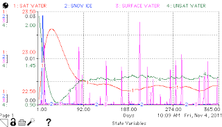
It does reach an equilibrium, and equilibrium levels of saturated water and unsaturated water are remarkably similar despite the four-fold difference in precipitation. What does change quite significantly is the amount of surface water (and snowpack):

Half precipitation

1x precipitation

Double precipitation

 The same patterns and equilibria hold when the simulation is run over three years.

3. Can you find a parameter in this model, modifying which you can produce a trend over several years that destabilizes the system?

First of all, I love these how-to-break-the-system questions.

Second, if we're given sufficient latitude with the parameters, the question becomes rather simple. Increasing transpiration potential by a factor of ten does little to the system; it remains stable at a very similar equilibrium; however, increasing the same parameter by a factor of 1000 sucks all the water right out of the system:

1000-fold increasing in transpiration potential

Ex 6.5 - Saturated soil zone dynamics

1. Why do the dynamics of unsaturated water look so much smoother in this model if compared to the model for unsaturated water only? 

In the unsaturated zone-only model, water that percolates out of the unsaturated zone is lost from the system. In the newer model, water that percolates out of the unsaturated zone enters the saturated zone. As a result, when precipitation falls and the site dries out, the unsaturated zone will recover water from the saturated zone, which will stabilize its levels. This wasn't possible in the older model because that water had left the system.

As evidence of this, notice that when precipitation falls, around day 200, percolation goes deeply negative and water moves from the saturated to the unsaturated zone. A miniature version of similar dynamics occurs again around day 600.

2. Can you make all the ground saturated and the unsaturated layer disappear from the system? What parameters need to be changed? What is their ecological meaning?

Is it just me or is this question, A) weird, and B) trivial?

 That said, you have to check the "non-negative" boxes for both stocks, to make this happen, but that's physically legitimate -- you can't have a negative amount of ground water.

Cranking transpiration up by an order of magnitude causes both stocks to go to zero within a year:

The ecological meaning of this is that plants are pulling more water out of the unsaturated layer, from whence it evaporates through their leaves, and the unsaturated water, in turn, sucks water from the saturated water, which then also ends up moving through the plants.

Ex 6.4 - Unsaturated soil zone dynamics

1. What other processes are important to define the flooding regime in the area? What paramters need to be changed to restore the drainage of the area and make sure that it does not get flooded? What ecological processes correspond to these changes in parameters? 

 There may be runoff from the site or movement of water out of the saturated zone, either of which would relieve flooding. Also, as the site gets wetter, the species composition of the vegetation of the site may change. The Gaia Principle suggests that the biota can regulate abiotic conditions to maintain them in the range that is suitable for life. Thus, as the site floods, plants with high transpiration rates may proliferate, removing water from the site in a nice feedback loop.

Finally, the amount of vegetation on the site will change with hydrological conditions. NPP stands for net primary productivity; it is the amount of carbon assimilated by an ecosystem per unit time. I have two issues with how NPP is incorporated in this model.

1. In the model, NPP is a defined dataset, changing only with the season, but in reality, NPP would change with the hydrological status of the site. When the site gets very dry, NPP declines. To a point, as the site moves closer to saturation, NPP increases, increasing transpiration (per the Gaia Principle), in a self-regulating feedback loop.
2. A more fundamental problem is that NPP is a rate, but it is used in the model as a stock. NPP is the rate of accumulation of biomass. But in modeling transpiration as NPP * transpiration rate (on a tissue-mass basis), NPP is being confused with plant biomass. That is, transpiration should be a function of standing biomass * transpiration per unit of biomass, not biomass added per unit time * transpiration per unit of biomass.

Incorporating those two changes could prevent the site from becoming totally saturated (flooded).

2. In fact when the Unsat_Depth decreases, certain amounts of unsaturated water get lost because they are no longer in the unsaturated zone. Imagine the water table rising and therefore the saturated water occupying more of the unsaturated zone. The unsaturated water in that marginal loss of the unsaturated depth will be lost from the Unsat_Water stock. Add this process to the Stella model. Is there a big difference in the results? 

Wow, this question took me way too much struggle, I think because I was confused by the units in the original model. Unsat_Depth sounds to me like it should be in meters, while Unsat_Water should be in cubic meters or liters, but to keep it simple the original model is all in depth. So, all I had to do was add this conditional to the percolation statement:

if Unsat_Water>Unsat_Depth
then (Unsat_Water-Unsat_Depth)*dt

Originally I had it as a seperate outflow from unsat_water, but then you could get outflow both due to percolation and the water table rising, which would be the same water leaving twice, so that's why I put it in the percolation, despite it making a fairly long conditional.

This change alters the behavior of the model very little because as the system is set up, unsat_depth is almost always greater than unsat_water. With different parameter values, though, it could make quite a difference.

Ex 6.3 - Snowpack-surface water model

1. Why do we model snowmelt as a constant rate rather than a proportion of the available snow? Make this modification to the model and analyze the difference in model performance. Which model seems to be more realistic? 

I don't know why snowmelt is modeled as a constant; perhaps because it's best to start with the simplest model possible and only add complexity when necessary. That said, if we want to make the snowmelt model more realistic, I would think that, in addition to total snowpack, temperature and incident radiation should be incorporated. Nevertheless, making snowmelt a function of the amount of snowpack, such that two percent of the snowpack melts on any day with temp > 0C (melt = 0.02 * snowice/dt) produces more realistic behavior than the constant snowpack model:

Melt as function of snowpack; note decay curve of "SnowIce."

2. Temperature in this model is presented as a random fluctuation over the sin function of time. What alternative methods could be used to generate temperature for this model? 

Weather station data could be used instead of a mathematical model. Incorporating not just average daily temperature, but also minimums and maximums, would likely improve the performance of the model.

6.2 - Evaporation model

1. As we have seen, our model of evaporation seems to produce less variability than the data (compare Evap_M and Hyd_evap_calc). Try to tweak the model parameters to increase the variability in model output.
 
All I did here was to augment the effect of cloudiness, and that seems to have brought the model's variability in line with the recorded data's. I changed SolRadGr from SolRad*(1-0.5*cloudy) to SolRad*(1-0.12*cloudy).

2. Check out the sensitivity of the model to changes in the parameter that describes the effect of cloudiness. What happens if the effect of clouds is increased quite dramatically (say, tripled)? How can we avoid some of the unrealistic behavior in the model that we observe in this case? 

By multiplying the parameter "cloudy" by three, we get hyper-dominance of cloudiness, such that on rather cloudy days, there's no evaporation:

We can avoid this behavior by not tripling the cloudy parameter. Just kidding. I think what he wants us to get at here is that by augmenting the effect of cloudiness within the SolRadGr function (as I did above), rather than augmenting the cloudy parameter itself, we can avoid the unrealistic behavior.


3. What is more important for the rate of evaporation: the latitude of the site, or the climatic conditions? What changes in climate can compensate the effect of the latitude and vice versa? 

Latitude has a relatively minor effect on evaopration:

LatDeg = 20 (model's minimum, in the tropics)

LatDeg = 64 (model's maximum, in the arctic)

On the other hand, we can see from the inter-dial and inter-seasonal variation that climatic conditions  exert a strong effect on evaporation. Although the following graph is crowded, it shows that air temperature is the primary driver of evaporation:

Ex 6.1 - Simple Surface Water Model

1. In Stella you can clamp your state variables to make sure that they never become negative. For example in this model the Surface_Water is non-negative. Note that the "non-negative" option is checked in the variable definition box. Since by default the variables get clamped in Stella this may be sometimes somewhat confusing and may hide some of the errors, when the variable is actually negative, but you do not see it. It is good practice to make sure that your processes (flows) are described properly, and do not deplete state variables beyond levels that are intended. Uncheck the non-negativity in this model and see what realy happens to the Surface_Water. Redefine the flows in the model to make sure that Surface_Water does not go negative. 


Obviously soil saturation is going to be a major determinant of the rate of surface water infiltration, but since we don't have a soil component in our model (yet, I hope), I just made infiltration a function of surface water: infiltration = .5 * surface_water

 
2. Let us supposed that the whole area got paved. How do we describe this in the model? What happens to Surface_Water? Does the result look plausible? Are there any other processes that we may be missing?

Assuming that the pavement is totally impermeable, surface water simply accumulates as the integral of rainfall. Obviously this is unrealistic, surface water will leave the site by flowing to lower elevations.

Ex. 5.3 - Trophic Chains

How does the model dynamics change if we consider the mortality process in the last model with the uptake of resource limited by the biomass in the first trophic level (N = u₀T₁)? Consider even and odd trophic chains and try to make some generaliztions. 

Well, the models' behaviors are interesting and quite divergent. Generalizations are going to be tough. Let's look at the three-trophic-levels model first. With death coefficient (d) = .05, the top predator dies off rapidly and the other two assume a periodicity that is reminiscent of the earlier predator-pray model.

Three levels, d = 0.05

If we decrease the mortality to d = .001, we get very different behavior. The first and third tropic levels decline, while the middle level enters a stable oscillation. I was curious how the system would collapse as levels 1 and 3 became extinct, so I extended the model to run to t = 1000, but the dynamics are unchanged. Levels 1 and 3 continue to decline, but are never eliminated, so level 1 continues to act as a conduit of "N" for level two.

Three levels, d = 0.001

Turning now to the four-level model, with d = .05, the overall behavior of the system is rather similar to the three-level model with d = .05 (the first set of graphs). There are some quantitative differences, but we see the same oscillations for the two lowest trophic levels (blue and red), and the highest (green) rapidly collapses.

4-levels, d = 0.05

In contrast, the four-level system with d = 0.001 exhibits very different behavior than the three-level system with d = 0.001. Whereas levels 1 and 3 declined in the three-level system, all four levels are stable in this system. Levels 1 and 3 oscillate roughly in-phase (lower-left scatter plot, note roughly direct proportionality), while levels 2 and 4 oscillate together, out-of-phase relative to levels 1 and 3.

4-levels, d = 0.001

Generalizations here are tough, but I'll try. One is that alternate trophic levels seem to move together, regardless of other details of the system, and adjacent trophic levels often move opposite each other. These are intuitive when we think in terms of top-down control: If there's a boom in coyotes, the will be a crash in rabbits, which will cause a boom in lettuce. In contrast, if we think in terms of bottom-up control, we wouldn't expect such behavior: a boom in lettuce will yield a boom in rabbits which will yield a boom in coyotes. Perhaps we can conclude that, at least for the system as we've formulated it, predator-based population controls dominate resource-based population controls. I wonder if I can turn down predation and turn up T1's resource use to make it not so... Indeed, just turning up u0, the first trophic level's source breaks the T1-T3 correlation. It also makes the system much flashier. Compare the above lower-left scatter plot, where when T1 is large, T3 is large and vise-versa, with the following lower-left scatter plot, where T1 and T3 appear to be inversely related. The only difference between them is the increased flow to the first trophic level (from 0.1 to 0.5).

And indeed, turning u0 up even further (to 1.0) strengthens the inverse relationship between T1 and T3. So perhaps we can conclude that when reourses at the bottom of the trophic web are abundant, they tend to govern the system, and when they are scarce, predation governs the system. That seems intuitive enough.

Ex. 5.2 - Predator-prey model sensitivity analysis

Run sensitivity analysis for this model with respect to the Half-saturation parameter SS. What do you observe when SS varies in the [0.5, 1.5] interval? How can you explain that?

Run 1 in red is SS = 0.5; run 5 in purple is SS = 1.5

As SS increases, the system converges toward the stable, non-trivial equilibrium more rapidly; that is, increasing SS dampens the extremes of rabbit and wolf populations as they approach their equilibrium values. The equilibrium populations are unaffected. This can be explained on several levels.

Mathematically, since SS is in the denominator of the predation function, as SS increases, predation slows, which effectively stabilizes the system.

Thinking about the system ecologically, if wolves consume rabbits very rapidly—that is, the slope of V vs. x is steep, which is a consequence of lower values of SS—then an increase in rabbit populations will produce a rapid upward swing in wolf population, because predation will increase their numbers before wolf mortality stabilizes their population. As a result of the increased number of wolves, the rabbit population will plummet, which will lead to a wolf die-off, and the cycle will repeat. On the other hand, when SS is large, predation is slow, so the wolf population reacts more gradually to fluctuations in the rabbit population, which effectively stabilizes both populations.

Exercise 5.1 - Modeling preditor-prey populations

1. Can you think of any examples of other systems that demonstrate the kind of behavior that we found in the predator-prey model?

Parasite-host dynamics are likely similar, where parasite population increases until the host’s capacity is reduced, at which point the parasite population declines until it finds a new host or the original host recovers to the point where the parasite can again expand.

2. In some predator-prey systems the prey can take refuge to hide from predators and avoid being consumed. Usually there is only a certain fixed number of individuals that the refuge can house. When the population of prey is large there is not enough refuge for all and the prey that could not find a place to hide gets consumed like in the standard predator-prey formalism. However when there are just a few preys their consumption slows down because they can find enough refuge places to hide. Build a predator-prey model with refuge and describe the dynamics that you observe. What equations did you modify and how? How can you explain the effect of refuge on the overall system dynamics?

To accomplish this, I made predation an exponential function:

V = y*a*e^b*x

Where V is predation, y is # wolves, x is # rabbits, and a and b are parameters that represent, respectively, the magnitude of the refuge available to the rabbits and how easily rabbits beyond the refuge are taken by wolves.

In general, this has the effect of stabilizing the system’s equilibrium. Effectively, the rabbit population is limited to the size of the refuge and the wolf population consequently limited by the size of the rabbit population. This causality can be seen reflected in the fact that the wolves’ curve reaches its asymptote slightly later than the rabbits’ curve.

Exercise 2.3 - Wizzles and Woozles

This is exercise 3.3 from the text, which is 2.2 online, and 2.3 in my nomenclature.

1. Consider a population of wizzles, which unlike woozles can multiply only when their numbers are larger than a certain minimal value a. If there are less byukies than a, they cannot find a partner for mating and the population dies off. The carrying capacity of the island where wizzles live is also A. Obviously A > a. What model would describe the population dynamics of wizzles on this island?

2. What are the equilibria in the byukies model? Are they stable? 

The solution that comes to mind isn't very satisfying, but it works. I've added an IF statement to the growth rate, such that if the A > a, the growth rate is positive, and if A < a, the growth rate is negative. The first image shows the model still works when the Ao > a; the second image shows the stable equilibrium at zero if the Ao < a.

Exercise 2.2 - Modeling a Toilet

A note on my nomenclature: This is exercise 3.2 from the text; it also happens to be 3.2 online, but online it's part of the art of modeling chapter, and in the text it's part of the math chapter. Following the online order, I'm calling the math chapter ch. 2, but since I'm working from the text for the math chapter (and only the math chapter) I'm calling this ex. 2.2. Whatever.

The model, as I downloaded it, needed to be broken before it could be fixed. First, I deleted the "/dt" from the outflow equation. Second, I changed the flush's if statement to be "if Use>0.995..." because I wasn't getting many flushes with the 0.999 threshold. Third, I deleted the seed from the random function ["RANDOM(0,1,14)" -> "RANDOM(0,1)"] in the parameter "use" to get different random flushings on each run. Doing that gives the following with dt = 0.5:

Q: Can you reformulate the model in such a way that the stock would be drained out properly under any computational method and any time step DT? As you may have noticed, when we switch to other methods, the outflow starts to deplete the stock, but then, apparently, does not have enough time to take it all out. How can this be fixed?

To get the tank to empty no matter what the dt, I just cranked up the outflow. Since tank is defined as a non-negative reservoir, this has no consequences. I made the outflow 1000 x tank, which should work up to a dt of 0.001. The result is: